In this post I claimed that the distribution in earnings of a NLHE 6-max cash player is essentially normal over a sample of at least thousands hands. I didn’t bother to justify my claim because I figured nobody cared. However, for those who do care, here’s a quick fudged argument and the real argument:
The Quick Argument
Here, I showed that large-field MTT earnings start to look normal after about 5k tournaments. The second table makes this fairly clear (though not particularly legible unfortunately). I think that it goes without saying that the distribution of earnings from one cash hand looks much more normal than the distribution of earnings from one large-field MTT. (In particular, the skewnessand kurtosis are much lower.) So, it seems pretty safe to assume that cash distributions are essentially normal over a few thousand hands.
This is the argument that I used to justify the use of the normal distribution to myself before making this post.
The Actual Data
Since it came up in the comments, I thought I’d actually check this directly. I grabbed the results from all my hands at NL200 6-max Rush on FTP, which turned out to be 54,250 hands with a winrate of 7.26 bb/100 and a SD of 116.97 bb/100. (I’m a huge lagtard when I play rush. Thus the high SD.) This isn’t the greatest sample in the world, but it’s fine for these purposes. Here’s that distribution, with normal distribution in red:
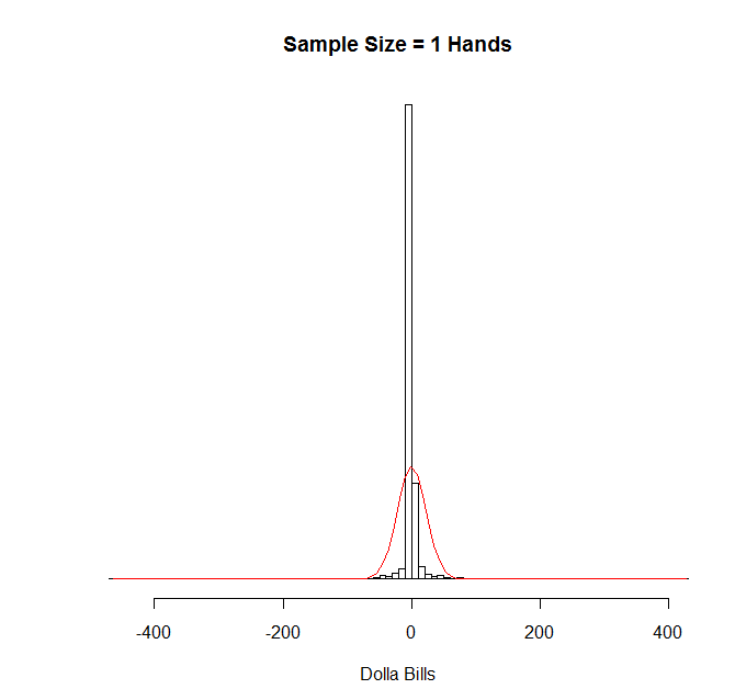
Obviously this is what you’d expect. The vast majority of the time I either earn $0 (the graph is centered in an odd way, so $0 looks negative), lose a little, or earn a little.
Here’s 100 hands:
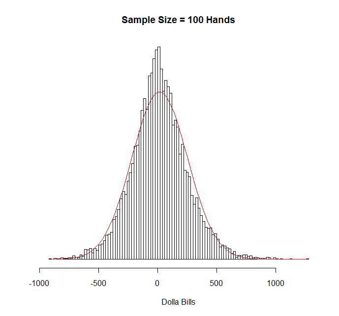
As you can see, it’s certainly not normal, but it’s gotten a lot closer. The (excess) kurtosis is about 1.1.
Here’s 1000 hands:
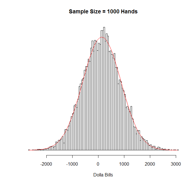
As you can see, that looks remarkably normal. The (excess) kurtosis is about 0.1 and the skewness is about 0.2. Not bad, eh?
Here’s 5000:
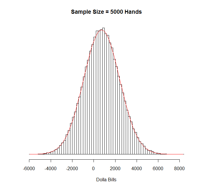
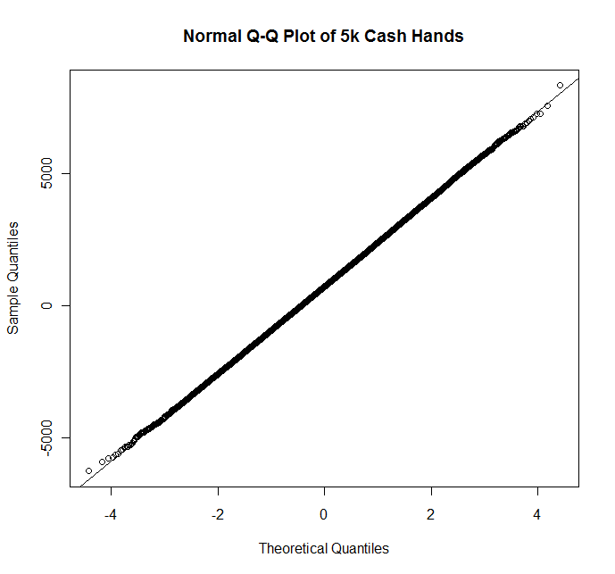
Now that’s a normal distribution. I could calculate the skewness and the kurtosis, but since I’m generating these things randomly, I doubt I’d be able to distinguish between this distribution and the normal distribution by that method. Here’s the Q-Q plot for completeness:
Noah,
Are the values in the graphs above generated using the stats from the hands in your database or are they measured from the actual sample? If they’re measured from the sample did you use a window (100, 1k or 5k) that overlaps hands at all?
When I pull the past 80k hands out of my HEM database, aggregate them into non-overlapping 100 hand chunks, and run the resulting 800 samples through excel I get an excess kurtosis of 2.6 (which may or may not be significant enough to impact tests that depend on normality).
I do know that using an overlapping window will cause problems (including the same hands in multiple samples introduces covariance into the data which will mess up results). If the results above were generated using the normal pdf this will cause problems as well (yeah, small random samples based on the normal distribution will quickly converge to the actual normal dist but that isn’t really what we’re interested in).
I’m more of a CS guy than a math guy so the way I’d end up approaching the problem is to take a large sample of hands, use that to create a histogram based on bb’s won/lost per hand and create a monte carlo sim based on that distribution.
You seem to have a stronger math background than I do so if you see anything wrong with my analysis or an easier way to crank this out let me know.
I didn’t use overlapping windows, or windows at all. I’m not 100% sure based on your description, but I think I did exactly what you said you would do.
I made a list (in R) of the results of my individual hands at NL200 Rush. I then randomly selected n results from that list (with replacement) and took the sum. I called this one sample. I rinsed and repeated 100,000 times and dropped the results in a histogram.
It’s possible that I’m making a significant mistake, but I don’t think I am. Obviously, using a sample of only 50k hands to generate the data isn’t ideal, but I doubt that would hugely change the results.
I don’t think that the kurtosis that you got necessarily contradicts mine since yours is only based on a sample of 800, so it could easily be random noise. Even if it did contradict mine, since kurtosis is proportional to 1/n, the kurtosis of a 5k-hand sample would still be ~.04 if your value for a 100-hand sample were correct. So, it doesn’t really matter much.
Regardless, I’m curious if your 80k hand sample includes a mixture of games and stakes. If that’s the case, that could explain your higher value, especially if you used consecutive hands in your sampling.
You did it exactly the way I was describing (the “with replacement” part).
I have a mix of 1/2 and 2/4 but I normalized the 80k hand sample to do the results in bb instead of $. Looking through my spreadsheet it looks like one of the hand buckets I have has a 450bb loss outlier in it. Removing that one outlier brings my value very close to yours.
Its been a good while since I’ve had to do anything with kurtosis but if it is proportional to 1/n (which would make sense given that the value I get when looking at individual hands is ~150) then yeah, even with a much higher value the effect is essentially nil.
Yeah. You could always run the same simulation that I ran on your data just to confirm that it looks normal above a 5k hand sample if you like. It doesn’t take very long.
(If you have R and an e-mail address, I’ll ship you my poorly-written code.)
“I made a list (in R) of the results of my individual hands at NL200 Rush. I then randomly selected n results from that list (with replacement) and took the sum. I called this one sample. I rinsed and repeated 100,000 times and dropped the results in a histogram.
“It’s possible that I’m making a significant mistake, but I don’t think I am. Obviously, using a sample of only 50k hands to generate the data isn’t ideal, but I doubt that would hugely change the results.”
Hi Noah,
Your methodology will of course converge to a normal distribution given a large enough sample due to the central limit theorem. However, the random sampling eliminates various factors that make real poker results non-random. Winrates are dynamic, as is volatility. Reasons for that include, but are not limited to:
a) game selection
b) quality of opponents
c) tilt
d) adjustments against regular opponents (as well as their adjustments)
e) developing your game (this can be positive or negative as you try new things)
The solution is to use non-overlapping “windows” as kerp hinted. I think you’ll find that using such a method will produce results that are significantly different than normal. Unfortunately this requires a much larger sample size for meaningful analysis (possibly more hands than any one person has ever played). But if you could get your hand’s on nanonoko’s or some other supergrinder’s data it would be super interesting.
While there’s no “correct” way to simulate this stuff, it would also be interesting to see how a variable winrate (say a winrate ranging from -2bb/100 to +10bb/100 between sessions with significant autocorrelation) and volatility clustering would change the distributions. You could attempt to look at empirical data to see what kind of assumptions you should make here, but I imagine it would be very difficult to extract anything you can be confident in.
Regardless, the end result is that cash game results should have fatter tails than the normal distribution implies. While this doesn’t really have significant consequences for the individual banrkoll management of a solid winner, it is something that can significantly affect the value of staking deals where the backer is often short a call option on the player’s results.
Petri,
Things like game selection and the quality of your opponents over the short term (say like a couple months) don’t affect these results at all. In essence, they make it so that instead of having a winrate of 4 bb/100, you have some spread of winrates each with thier own weight that average to 4 bb/100. For example, you might have 0 bb/100, 2 bb/100, 4 bb/100, 6 bb/100, or 8 bb/100 with equal weightings. Statistically, though, that’s the same thing. Your winrate is still 4 bb/100 on average, and you can still treat every time that you sit down at a table as creating a random variable with mean of 4 bb/100 and sd of whatever your sd is (usually around 80-100 bb/100 at 6-max NLHE). So you’re still just summing up independent random variables with identical means and standard deviations, and the central limit theorem still applies.
Indeed, the same is true for long-term changes, though the argument is slightly more complicated. If I expect that a player is going to play n_i hands with a winrate of i bb/100, it obviously doesn’t matter what order they’re played in, and over a relatively significant sample size, I can replace this by giving the player an n_i/n chance of having an i bb/100 winrate in any given hand. Those obviously will have near identical distributions provided that the sample size is large enough that n_i/n chance run n times will hit about n_i times with near certainty. By using that (very very justified) approximation, the central limit theorem still applies. So, change in winrate over time does not result in fat tails, and all the statistics I’ve done still works. So, that takes care of long-term changes in player pools and long-term adjustments by both you and your opponents.
Of course, actually estimating these distributions is basically impossible statistically, but so is estimating your winrate in the first place. Estimating your winrate requires guess work, as does estimating how it will change over time. If I were a backer, I would obviously choose the worst case scenario before agreeing to back somebody; For example, at NLHE 6-max, I would estimate his winrate and then lower the estimate by, say, 2 bb/100 and crunch the numbers with that.
Tilt obviously screws things up because it means that the variables are no longer independent, so the normal distribution no longer applies. I’m going to do a post on that at some point. If you’re a backer, don’t back somebody with a tilt problem. If you’re a player, don’t have a tilt problem….
Noah,
What you’re saying is true if you assume that changes in winrate and standard deviation are random. This isn’t the case – they are autocorrelated. You seem to have recognized this re:tilt but it applies the same for the other factors I mentioned.
If you’re taking the numbers from HEM/PT I imagine they calculate SD on a hand by hand basis and then scale it by assuming independence between hands. This will underestimate the actual standard deviation.
“Tilt problems” are also unavoidable with human players. They might range from full blown monkey tilt to minor things like being slightly more timid when running extremely bad. But unless you’re running a bot, it will be a source of autocorrelation in results that for almost all players will make the actual standard deviation higher than that predicted by scaling the SD/100 stat from HEM.
I didn’t assume that changes are random, I showed that they’re effectively equivalent to random changes.
HM/PT do calculate standard deviation in that way, and that is the correct way to calculate it.
I suppose you’re right that tilt is basically unavoidable. I would argue that the minor effects that you talk about (which are the norm for players who are able to be successful) are minor enough to not influence the results signfiicantly. I suppose I have no proof of that, but it seems fairly obvious to me. It’s certainly the case that if your winrate drops by, say, 2 bb/100 when you’re tilting, your distribution can’t be any worse than a player with a constant winrate that is 2 bb/100 less than your average.
If tilt did significantly affect a player’s distribution, it would not change the calculated standard deviation (SD just has a mathematical definition, and there’s only one way to calculate it), but it would change the distribution to one with fatter tails than the normal distrubution.
Again, I plan on writing up a post about this at some point (perhaps a month from now when I’ve banged out a few more Life as a _____ Pro posts and am less busy with RL stuff), so I’ll have much more to say then.
I didn’t assume that changes are random, I showed that they’re effectively equivalent to random changes.
I’d argue that you haven’t shown this. While it is true that for very large samples the sum of a series of autocorrelated variables (distribution of total money won over say 10M hands played under the same conditions) will converge to the normal distribution implied by the HEM SD figure, the autocorrelation caused by the factors I mentioned previously (among others) will make the required sample size very large. The question is “how large?” This could really only be determined by a very large empirical study, and it would vary greatly from player to player. A rush poker grinder’s results (low autocorrelation) would converge a lot faster than a HU bumhunter’s (extremely high autocorrelation), for example.
If tilt did significantly affect a player’s distribution, it would not change the calculated standard deviation (SD just has a mathematical definition, and there’s only one way to calculate it), but it would change the distribution to one with fatter tails than the normal distrubution.
I think you missed my point here. A player with an SD of 100bb/100 according to HEM may have a true SD for a sample of 10k hands in the range of 1050-1300bb rather than the 1000bb that would be implied by simply scaling the bb/100 figure. Being prone to tilt would push it toward the high end.
Hi Petri,
I have an exam tomorrow that I need to study for, so I won’t be able to give you the long response that you deserve until after my exam.
The cliffs is that I’m quite sure that you’re right with regard to tilt, and I’m quite sure that the rest of your points are wrong. I think that you’re confusing correlation between means and correlation between results independent of means. There’s an important difference there, and I’ll rant about it ad nauseum tomorrow evening. (Please remind me via e-mail if I forget.)
-Noah
Woops, I believe the first part of my last post is incorrect. Will expand later.
“I think that you’re confusing correlation between means and correlation between results independent of means”
I can see why you would think this based on the first part of my previous post as it was very poorly worded (and is in fact incorrect the way it was written). I’d delete/edit that part of the post if I could… feel free to do so if you like.
Regardless, the correlation between means and standard deviations causes a correlation between results and their standard deviations that I don’t believe to be insignificant over reasonable samples, say 100k hands. Aside from tilt, other huge factors would be getting a big fish heads up (this could easily increase your winrate by 10bb/100 over say 5k hands). Even in high stakes 6max games having a big fish play in the games for a while could easily increase one’s winrate by 5bb/100 for say 5k hands; increasing your expectation by 250bb over a 100k sample is pretty huge if your “normal” expectation is, say 1bb/100 or 1000bb.
The majority of us (perhaps not you rush poker grinders :P) make significant changes and experiment with our games on a regular basis – things like this could easily increase or decrease our winrates for long periods of time. Having an opponent find a leak that he exploits you with over 20k hands before you notice it could kill your EV. Going through a stretch of often playing bored/unfocused/tired could have a huge effect. There’s countless factors that could potentially cause significant long term fluctuation and correlation in expected winrates.
I don’t know how much cash game data you’ve been able to collect, but if you could look at actual played hands in 10k (or bigger if you have the data) chunks and compare the distributions you find to those predicted by scaling the HEM SD/100 figure, I think you’ll find a greater standard deviation of results than you’d expect. This will be even more true if you use a forward-looking prediction of winrate rather than the in-sample data.
Yeah.. I think we were talking past each other a bit, and I now think I have a good sense for what you’re saying.
Indeed, use of the central limit theorem to describe real-world processes is risky business, and even though using it is pretty simple, knowing when it will work well and when it will result in completely incorrect results is a pretty damn difficult problem in general. I do think that I’m justified here, but you raise some important concerns.
Again, I’ll write up an appropriately long response to your questions tomorrow evening. Please bug me if I forget.
Hi Petri,
So I think there are a few separate arguments here. I’ll list them roughly from strongest to weakest. (I apologize if I’m misunderstanding you and putting words in your mouth):
Hope that clarifies.